Floquet theory
Floquet theory is a branch of the theory of ordinary differential equations relating to the class of solutions to linear differential equations of the form

with  a piecewise continuous periodic function with period
  .
.
The main theorem of Floquet theory, Floquet's theorem, due to Gaston Floquet (1883), gives a canonical form for each fundamental matrix solution of this common linear system. It gives a coordinate change  with
with 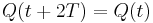 that transforms the periodic system to a traditional linear system with constant, real coefficients.
In solid-state physics, the analogous result (generalized to three dimensions) is known as Bloch's theorem.
Note that the solutions of the linear differential equation form a vector space. A matrix  is called a fundamental matrix solution if all columns are linearly independent solutions. A matrix
  is called a principal fundamental matrix solution if all columns are linearly independent solutions and there exists
  such that
  is the identity. A principal fundamental matrix can be constructed from a fundamental matrix using
 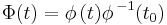 . The solution of the linear differential equation with the initial condition
  is
is 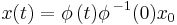 where is any fundamental matrix solution.
Contents |
Floquet's theorem
Let  be a linear first order differential equation, where
  is a column vector of length
  and
and  an
an  periodic matrix with period (that is
 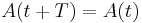 for all real values of
  ). Let be a fundamental matrix solution of this differential equation. Then, for all
  ,
,
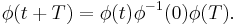
Here
is known as the monodromy matrix. In addition, for each matrix  (possibly complex) such that
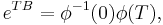
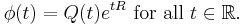
there is a periodic (period ) matrix function  such that
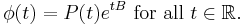
Also, there is a real matrix  and a real periodic (period-
 ) matrix function
  such that
In the above ,  ,
,  and are matrices.
Consequences and applications
This mapping 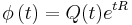 gives rise to a time-dependent change of coordinates (
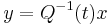 ), under which our original system becomes a linear system with real constant coefficients
  . Since
  is continuous and periodic it must be bounded. Thus the stability of the zero solution for
  and is determined by the eigenvalues of .
The representation 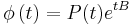 is called a Floquet normal form for the fundamental matrix .
The eigenvalues of  are called the characteristic multipliers of the system. They are also the eigenvalues of the (linear) Poincaré maps
 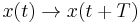 . A Floquet exponent (sometimes called a characteristic exponent), is a complex
  such that
  is a characteristic multiplier of the system. Notice that Floquet exponents are not unique, since
 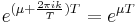 , where
  is an integer. The real parts of the Floquet exponents are called Lyapunov exponents. The zero solution is asymptotically stable if all Lyapunov exponents are negative, Lyapunov stable if the Lyapunov exponents are nonpositive and unstable otherwise.
- Floquet theory is very important for the study of dynamical systems.
- Floquet theory shows stability in Hill differential equation (introduced by George William Hill) approximating the motion of the moon as a harmonic oscillator in a periodic gravitational field.
Floquet's theorem applied to Mathieu equation
Mathieu's equation is related to the wave equation for the elliptic cylinder.
Given  , the Mathieu equation is given by
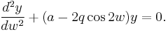
The Mathieu equation is a linear second-order differential equation with periodic coefficients.
One of the most powerful results of Mathieu's functions is the Floquet's Theorem [1, 2]. It states that periodic solutions of Mathieu equation for any pair (a, q) can be expressed in the form
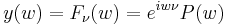
or

where  is a constant depending on a and q and P(.) is
  -periodic in w.
The constant is called the characteristic exponent.
If is an integer, then  and
and  are linear dependent solutions. Furthermore,

for the solution or , respectively.
We assume that the pair (a, q) is such that 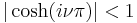 so that the solution
  is bounded on the real axis. General solution of Mathieu's equation (
 , non-integer) is the form

where  and
and  are arbitrary constants.
All bounded solutions --those of fractional as well as integral order-- are described by an infinite series of harmonic oscillations whose amplitudes decrease with increasing frequency.
Another very important property of Mathieu's functions is the orthogonality [3]:
If  and
and  are simple roots of
then:
i.e.,

where <.,.> denotes an inner product defined from 0 to π.
References
- C. Chicone. Ordinary Differential Equations with Applications. Springer-Verlag, New York 1999.
- Ekeland, Ivar (1990). "One". Convexity methods in Hamiltonian mechanics. Ergebnisse der Mathematik und ihrer Grenzgebiete (3) [Results in Mathematics and Related Areas (3)]. 19. Berlin: Springer-Verlag. pp. x+247. ISBN 3-540-50613-6. MR1051888.
- Floquet, Gaston (1883), "Sur les équations différentielles linéaires à coefficients périodiques", Ann. École Norm. Sup. 12: 47–88, http://archive.numdam.org/ARCHIVE/ASENS/ASENS_1883_2_12_/ASENS_1883_2_12__47_0/ASENS_1883_2_12__47_0.pdf
- Krasnosel'skii, M.A. (1968), The Operator of Translation along the Trajectories of Differential Equations, Providence: American Mathematical Society, Translation of Mathematical Monographs, 19, 294p.
- W. Magnus, S. Winkler. Hill's Equation, Dover-Phoenix Editions, ISBN 0-486-49565-5.
- N.W. McLachlan, Theory and Application of Mathieu Functions, New York: Dover, 1964.
- Teschl, Gerald. Ordinary Differential Equations and Dynamical Systems. Providence: American Mathematical Society. http://www.mat.univie.ac.at/~gerald/ftp/book-ode/.
- M.S.P. Eastham, "The Spectral Theory of Periodic Differential Equations", Texts in Mathematics, Scottish Academic Press, Edinburgh, 1973.